Mirrorless Metering

Gary Hart Photography: Dawn Reflection, Trillium Lake and Mt. Hood, Oregon

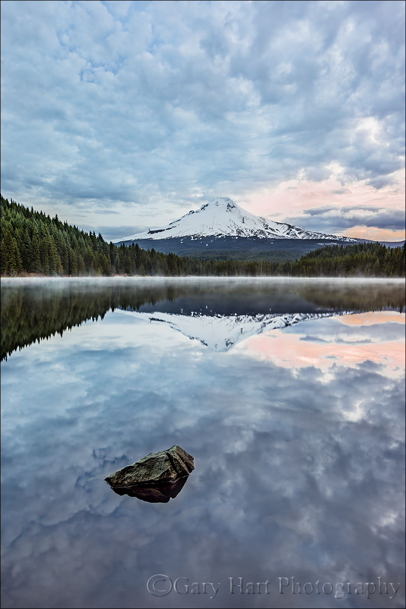
Morning Peace, Trillium Lake and Mt. Hood, Oregon
Sony a7R
Sony/Zeiss 16-35 f/4
.5 seconds
F/11
ISO 100

Once upon a time, to ensure perfect exposure, photographers had to carefully meter their scene before clicking, after clicking we had to wait until we completed the roll, return home, send the film off to the lab, and cross our fingers waiting for its return. We’d sometimes hedge our bets by bracketing, but that cost time and money, only worked when the subject was stationary, and didn’t insure against an egregious exposure error. For many the exposure techniques from the film days carry over to this day (it took me many years to shake them), but there really is an easier way. It starts with what I’d call the single most significant benefit to digital capture: the histogram.

Trust your histogram

The histogram is a graph of the tones in an image (you can read more about it here). Instead of clicking and hoping as we did in the film days, the addition of a histogram on every digital camera gave photographers instant feedback on the image’s exposure. Better still, live-view histograms give us that exposure feedback before clicking the shutter.

Setting up your live-view histogram

To ensure a valid pre-capture histogram (on your DSLR’s live-view screen, or your mirrorless camera’s live-view or viewfinder screen), make sure you are in whatever your camera manufacturer calls exposure simulation. When the camera simulates exposure, rather than always showing the ideal exposure on the live-view screen, it attempts to emulate the exposure settings you’re using. Here is an incomplete and far from comprehensive guide to the terminology used by the major camera manufacturers.

Canon: Exposure Simulation (enabled)
Fuji: Preview Exp. in Manual Mode (off)
Nikon: Exposure Preview (selected in the Info menu)
Olympus: Live-view Boost (off)
Sony: Setting Effect (on)

While each camera manufacturer offers a variety of metering mode options and terminology to label them (spot, partial, center-weighted, evaluative, matrix, etc.), your metering mode doesn’t matter if you’re metering with your histogram.

Once you’ve turned on exposure simulation, you need to figure out how to display the histogram while metering. Most cameras, mirrorless or DSLR, offer multiple live-view screen options that display a variety of information about the scene you’re photographing. On most cameras, only one of these screens displays the histogram—finding it is usually a simple matter of cycling through the various displays until the histogram appears—to minimize the number of screens I need to scroll through to see the information I need (such as the histogram or level), I always go into my camera’s menu system and disable the live-view screens I don’t use.

Using your live-view histogram

Using the pre-capture histogram, I start the metering process as I always have, using my camera’s best ISO (100 for my Sony a7RV), and the best f-stop for my composition (unless motion, such as wind or star movement, forces me to compromise my ISO and/or f-stop). With ISO and f-stop set, I slowly adjust my shutter speed with my eye on the histogram in my viewfinder* (or LCD) until I’m satisfied with the histogram. Ideally I’ll have a little room on both sides of the histogram, but in a high dynamic range scene my histogram might not fit the boundaries, in which I usually add exposure until the histogram graph bumps against the right side.

Most mirrorless bodies offer highlight warnings in their pre-capture view (called “zebras” on my Sony bodies). While these alerts aren’t nearly as reliable as the histogram and should never be relied on for final exposure decisions, I use their appearance as a signal that it’s time to check my histogram. The first time I meter a scene, my current exposure settings (based on my prior scene) can be far from what the current scene requires—in this case, I push my shutter speed fast until the zebras appear (if my prior exposure was too dark) or disappear (if my prior exposure was too bright), then refine the exposure more slowly while watching the histogram.

In a low or moderate contrast scene, I’ll have a little room on both sides of the histogram—a pretty easy scene to expose. But in a high dynamic range scene, the difference between the darkest shadows and brightest highlights might stretch the histogram beyond its boundaries. When a high dynamic range scene forces me to choose between saving the highlights or the shadows, I almost always bias my exposure choice toward sparing the highlights, carefully dialing the exposure until the histogram bumps against the right side.

Because the post-capture histogram is more reliable than the pre-capture histogram, when there’s little margin for error, I verify my exposure by checking the post-capture histogram. Here’s where the RGB (red, green, blue) histogram becomes important. While the luminosity (white) histogram gives you the detail you captured, it doesn’t tell you if you lost color. Washed out color is always a risk when you push the histogram all the way to the right, so it’s best to check the post-capture RGB histogram to ensure that none of the image’s color channels are clipped.

An often overlooked aspect of mastering in-camera metering is simply learning how your camera reports exposure. Not only does every camera interpret and display its exposure information differently, the histogram returned is based on a jpeg, so raw shooters always have more information than their camera reports—it’s important to know how much more. With my Sony a7R-series bodies, I know I’m usually safe pushing my histogram’s exposure graph up to a full stop beyond the left or right (highlights and shadows) boundary—I have no problem using every available photon.

For example

Dawn Reflection, Trillium Lake and Mt. Hood, Oregon

A few years ago I was photographing a sunrise at Trillium Lake, beneath Mt. Hood and just south of the Columbia River Gorge. Finding the open sky on Mt. Hood’s east side much brighter than the lake and (especially) trees, after composing and focusing, I cranked my shutter speed until the zebras appeared (they usually show up before the histogram reaches the right side), then clicked more deliberately until the histogram hit the right side.

At that point the left side of the histogram was still clipped slightly, but because I knew I still had one more stop to play with on the highlights side, I clicked one more time with my eye on the left (shadows) side of the histogram and saw that the shadows were still slightly clipped. Since each click adds (or subtracts) 1/3 stop, I had two more clicks before I reached my 1-stop-over highlight threshold. The second shutter-speed click moved the left side of the histogram just enough to eliminate the clipped shadows, and I was ready to shoot (with 1/3 stop to spare!).

After capture, I checked my RGB histogram to ensure that I’d captured all the scene’s detail and color. In Lightroom I was able to easily recover the highlights that my camera told me were clipped, and pull all the detail I needed from the shadows.